Understanding Landsat Collections, Levels and Tiers – which do I use?

      Monday 17 January 2022 |  by Kris Chan

      Category: Satellites

Collections? Levels? Tiers? Landsat’s data processing classification is confusing to say the least and will trip up the unwary. With some typologies due to be discontinued in future, it is imperative you use the correct type. Here, I’ll break down what you need to know.

***Precursory notice: This a preliminary (/emergency) post to help students ensure they are using the best current Analysis Ready Data and that they are future-proofing their work. The post will be expanded in due course, once I have more time to devote to explaining the nuances of the different terms, details of future changes, and explanations of why the three broader classifications exist (spoiler: it is really to make our lives easier in the future).***

Which do you generally recommend?

Short answer: if you plan to use the best pre-processed (Surface Reflectance) Landsat data, it currently (Jan 2022) needs to be:

• Collection 2
• Level 2
• Tier 1

For those using EarthEngine, the specific imageCollection for this of Landsat 8 is:

ee.ImageCollection(“LANDSAT/LC08/C02/T1_L2″)

To attain this for the other Landsat satellites, change LC08 of the above to: LE07 (for Landsat 7), LT05 (for Landsat 5), and LT04 (for Landsat 4).

The nuances of the naming conventions are confusing and may be liable to change. As of January 2022 however, the above is very much the recommended data types (for pre-processed surface-reflectance data).

Note however that for some images, the processing of existing datasets to these may not currently be complete, and due to the stricter data quality requirements of the higher quality data (of Collection 2, Level 2, Tier 1 data), there will consequently be less suitable images over time than if you were to select a lower quality level of data. To put it another way, if you prioritise understanding finer-scale season changes over more accurate and long-term changes, you may want to opt for a lower classification of data.

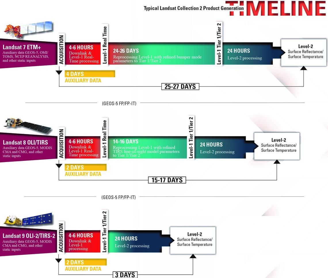
Similarly, if you required the most recent satellite data (i.e. <25-27 days old for Landsat 7, <15-17 days for Landsat 8, <3 days for Landsat 9 – see image below), you will be limited to Level 1 (non-surface reflectance and potentially non-geometrically corrected) data. Using such ‘raw’ data is not a trivial undertaking, and we would recommend you do not embark on using this unless you really can’t avoid doing so. You should also have a very strong understanding of the different corrections to understand if and how to perform some of these corrections yourself.

Specific information about Collection 2 data you should know

Collection 2 data is only available for Landsat satellites 4-9

Previous Landsat satellites carried a much simpler sensor (a 6-bit system for a maximum of 64 separate brightness values and spatial resolution of just 60m) and sufficient data of the location-specific atmospheric condition at the time of satellite overpass is generally insufficient to produce data of sufficient accuracy to meet the collection 2 requirements. Really, unless you are performing more qualitative analysis or are familiar with the complexities of Landsat 1-3, we generally recommend you restrict your analysis to Landsat 4 and after, (~1982 onwards).

Collection 1 data processing has stopped, and data is expected to be unavailability in future

The main reason for advising for the use of Collection 2 data, NASA announced that as of 1 January 2022, all new Landsat scenes acquired will only be processed via Collection 2’s workflow. NASA have furthermore only committed to hosting Collection 1 data until 31 December 2022. It should be noted that Google perform their own processing of much of the data collected via the Landsat programme, though whether this will include Collection 1’s workflow remains to be seen (don’t bet on it!).

Collection 2 scaling of pixel values is much more complicated

An important caveat of using Collection 2 data is the different scaling used to transform pixel values to meaningful reflectance values.

Rather than the previous shorthand of multiplying the pixel value by 0.0001 (or conversely, dividing by 10 000), the scaling of pixel values involves both a scaling factor and offset. This makes conversion from the pixel values to actual reflectance much more difficult, particularly for checking mentally.

Let’s say your Collection 2, Level 2, Tier 1 pixel now is a value of 15 432. To calculate actual surface reflectance you must first multiply this pixel value by the scaling factor (0.000 0275) then add the offset (-0.2). Let’s demonstrate that now:

Thus, our pixel value of 15 432 provides a reflectance of 0.22438 (or 22.438%). Those mathematically minded can perform a quick quality check as 15 432 is ~1/5 between 7273 (the approximate new pixel value for a reflectance of 0) and 43 636 (the approximate new pixel value for a reflectance of 1).

Knowing the techical 0 and 1 reflectance values (7272.72…. and 43636.36…. respectively) we could also calculate the true reflectance by first minusing the new accurate 0 reflectance value, then dividing by the new range between the 0 and 1 value (i.e. 36363.63….). We’ll demonstrate that below:

The first method is recommended when actually calculating real reflectance values, not least due to the complication of recurring values with the second method. I however thought it worthwhile to mention the second method as another way to potentially help think about how to mentally recalculate the values.

Why was the scaling changed?

Ultimately to provide greater accuracy of the data. Rather than being limited to 10,000 independent values between a reflectance of 0-1, we instead have 36,364 values, meaning over three times the precision. Confusingly however, the original satellite data will probably not have had this level of precision; Landsat 8’s sensor was 12-bit (4096 total values) and Landsat 4-7 was 8-bit (256 total values). That said, by having a greater resolution of post-processed data, reflectance values can more accurately reflect what the original calculated values were.

Collection 2 data cannot be immediately merged with collection 1 data

This is both due to the scaling factors, in addition to the different metadata formats of the different collection types.

Collection 2 data is more readily comparable to Copernicus/Sentinel satellite data

A major reason for the reprocessing of the Landsat time-series to Collection-2 is to facilitate better cross-satellite comparison.

There are many, many differences in processing which lead to the different designations

A table summarising the specific differences between different Collection 1/2 and Level 1/2 data can be found here, or a more easily digestible version can be found under the “Collection 2 Highlights” heading here. Differences include what atmospheric correction algorithms are used, the specific data that feeds into these, the geographic precision of the data and what data is used to correct for this, whether the data is more aligned/readily comparable with Sentinel and other satellites, whether stray light is corrected for, etc. Explaining all of the differences of these and keeping this information accurate and up-to-date is really beyond the scope of this blog. Rather, the purpose of this blog is to attempt to relay key information necessary to allow yourselves to quickly understand the more general differences between the terminologies and which you should use.

Future updates:

I will add further explanation to this in future (together with the justification of why these changes are/have been implemented), but as of January 2022, if you want the most accurate calibrated surface reflectance data, use Collection 2, Level 2, Tier 1 Landsat data.